Developer’s corner #

Contents

Developer’s corner

Tools for computer programmers including FDSNWS and UDP Streaming #

UDP data streaming #

See Raspberry Shake Data Producer UDP Port Output

Scripting language tool-boxes (MATLAB and Python)#

These MATLAB and Python toolboxes are useful for programmers who want to create their own data visualization or processing routines.

MATLAB: GISMO

Python: Obspy

Contributed software #

Raspberry Shake on GitHub #

Raspberry Shake Community GitHub Account

sl2influxdb #

sl2influxdb by Marc Grunberg on GitHub

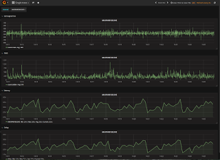
Description: Dump seedlink (seismological) time series into InfluxDB. Use Grafana to plot waveforms, real time latency delay, etc. Maps uses the grafana worldmap-panel plugin.

seisplotjs #

seisplotjs by Phillip Crotwell on GitHub

Description: Javascript modules for parsing, manipulating and plotting seismic data.

Phillip says,

“Also included in this (and available separately) is seisplotjs-filter for basic waveform filtering, and seisplotjs-traveltime that queries the IRIS traveltime web service (which internally uses my java travel time calculator, TauP) as well as seisplotjs-distaz which will do the spherical distance calculations without a web call and seisplotjs-fdsnevent that queries a web service for event parameters. There are others as well, so anything in my github that starts with “seisplotjs-” is (or will be) part of this. Here are a bunch of links for your clicking pleasure…

seisplotjs-waveformplot

seisplotjs-filter

seisplotjs-traveltime

seisplotjs-distaz

seisplotjs-fdsnevent

Also some of the examples that may be useful are here. This should be the same as the corresponding github code, just with the dependencies and so runnable.

All free for reuse, but under active development so expect missing documentation, wrong examples and probably lots of changes as I improve it, :) but I hope it will be useful. The goal is to eventually be able to do basic seismic data processing in the browser without relying on any server-side coding.”

Converting counts to metric units using ObsPy #

Many users will want to convert the output from their Raspberry Shake to real-world (metric) units. There are several programs that can do this, including the Swarm GUI. In this example, we will use the ObsPy seismological library for Python to convert from counts to acceleration.

Note

This example will work “out-of-the-box” if your Shake is forwarding data to our servers. If it is not forwarding data to our servers, obspy will need a different source from which to download your Shake instrument response.

In this case, we provide Templates for manual metadata generation from which you can adapt a template of your own station’s instrument response manually (i.e. find and replace the placeholder with your own station name in the metadata file corresponding to your Shake version).

The output of every Raspberry Shake device is counts, a unitless number that is essentially an analogue for the amount of voltage on the circuit of the given channel at the given time.

This example will create two plots, first with raw counts, and second with deconvolved units:

from obspy.clients.fdsn import Client
from obspy.core import UTCDateTime, Stream
rs = Client('RASPISHAKE')

# set the station name and download the response information
stn = 'R24FA'                            # your station name
inv = rs.get_stations(network='AM', station=stn, level='RESP')

# set data start/end times
start = UTCDateTime(2020, 3, 7, 2, 40, 45) # (YYYY, m, d, H, M, S)
end = UTCDateTime(2020, 3, 7, 2, 42, 0) # (YYYY, m, d, H, M, S)

# set the FDSN server location and channel names
channels = ['EHZ', 'ENE', 'ENN', 'ENZ'] # ENx = accelerometer channels; EHx or SHZ = geophone channels

# get waveforms and put them all into one Stream
stream = Stream()
for ch in channels:
        trace = rs.get_waveforms('AM', stn, '00', ch, start, end)
        stream += trace

# here you will plot raw counts for all four channels
stream.plot()

# attach the response info
stream.attach_response(inv)

# remove the response and plot
resp_removed = stream.remove_response(output='ACC') # convert to acceleration in M/S/S

# now plot all channels in acceleration units (m/s/s)
resp_removed.plot()

Converting counts to Pascal to Decibel using ObsPy #

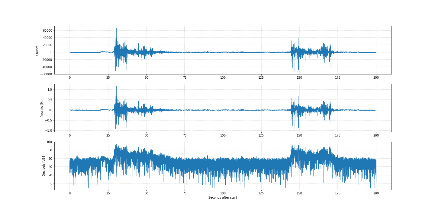
Continuing from the previous section, it is possible that RBOOM and RSBOOM users will want/need to convert the pressure transducer sensor output in counts to Pascal (the standard atmospheric pressure unit) or even to Decibel. It is possible to do so using again the ObsPy seismological library for Python, with this step-by-step guide.

Note

This example consists in a very basic code and it is pre-set on two thunder events registered in 2018 by the R796B Shake. If your Shake is not forwarding data to our servers, obspy will need a different source from which to download your Shake instrument response.

As stated, the output of every Raspberry Shake device is counts, a unitless number that is essentially an analogue for the amount of voltage on the circuit of the given channel at the given time.

This example will create a single plot with three subplots: raw counts, pascal, and decibel.

from obspy.clients.fdsn import Client
from obspy import UTCDateTime
import matplotlib.pyplot as plt

# define start and end times
start = UTCDateTime(2018, 8, 4, 15, 4, 40) # (YYYY, m, d, H, M, S)
end = UTCDateTime(2018, 8, 4, 15, 8, 0) # (YYYY, m, d, H, M, S)

# define fdsn client to get data from
client = Client('http://data.raspberryshake.org')

# get data from the FSDN server and detrend it
STATION = 'R796B'               # station name
st = client.get_waveforms('AM', STATION, '00', 'HDF', starttime=start, endtime=end, attach_response=True)
st.merge(method=0, fill_value='latest')
st.detrend(type='demean')

# set-up figure and subplots
fig = plt.figure(figsize=(20,10))
ax1 = fig.add_subplot(311)
ax2 = fig.add_subplot(312)
ax3 = fig.add_subplot(313)

# plot the three curves
ax1.plot(st[0].times(reftime=start), st[0].data, lw=1)
ax2.plot(st[0].times(reftime=start), (st[0].data/56000), lw=1)
ax3.plot(st[0].times(reftime=start), 20*np.log10(abs(st[0].data/56000)/0.00002), lw=1)

# set-up some plot details
ax1.set_ylabel('Counts')
ax2.set_ylabel('Pascals (Pa)')
ax3.set_ylabel('Decibels [dB]')
ax3.set_xlabel('Seconds after start')

ax1.grid(color='dimgray', ls = '-.', lw = 0.33)
ax2.grid(color='dimgray', ls = '-.', lw = 0.33)
ax3.grid(color='dimgray', ls = '-.', lw = 0.33)

# save the final figure
plt.savefig('dBPlot_test.png')

Table of Contents

Developer’s corner