Example Data

Example 1: GSN station KIP

Description: 20 days of LHZ (1 sps) data from 2 co-located broadband sensors:

1. “Known” instrument: a Streckeisen STS-1VBB w/E300 (00_LHZ.512.seed; RESP.IU.KIP.00.LHZ); and
2. “Unknown” instrument: a Streckeisan STS-2.5 (10_LHZ.512.seed, RESP.IU.KIP.10.LHZ).

The Streckeisen STS-1VBB has a flat frequency response that extends to lower frequencies and, therefore, is used in this example to determine the frequency response of the more band-limited STS-2.5. Data was provided by Adam Ringler of the Albuquerque Seismic Laboratory. A full station description can be found at http://www.iris.edu/mda/IU/KIP.

Note

The GSN network has MANY MANY co-located sensors and therefore served as an EXCELLENT source of test data for respGen.

First, configure /opt/osop/respgen/setup.py in this way:

#!/usr/bin/env python2
UFILE = 'DATA/10_LHZ.512.seed'
KFILE = 'DATA/00_LHZ.512.seed'
URESP = 'DATA/RESP.IU.KIP.10.LHZ'
KRESP = 'DATA/RESP.IU.KIP.00.LHZ'
OVERLAP_FRACTION = 0.8
NUM_OF_WINDOWS = 100
LOWFRQ = 0.0001
NUM_OF_POINTS = 1500
MEDIAN_LEN = 7
COHE_LIMIT = 0.6
DETERMINE_DEGREE = True
NMAX = 6
NN = 4
MM = 3
NORMFREQ = 0.1
ZERO_LIMIT = 0.0015

Then, execute view_cohe.exe:

# view_cohe.exe

The terminal output should be:

# view_cohe.exe

Coherence of the inputs

Input from the known instrument:
DATA/00_LHZ.512.seed

Input from the unknown instrument:
DATA/10_LHZ.512.seed

Reading input data.
Truncating inputs to the overlapping time.
Determining the length of the window

Will use window length: 4096 (2**12)
Will use frequency range: [0.000122, 0.500000]

Removing DC from both input arrays.
Calculating coherence

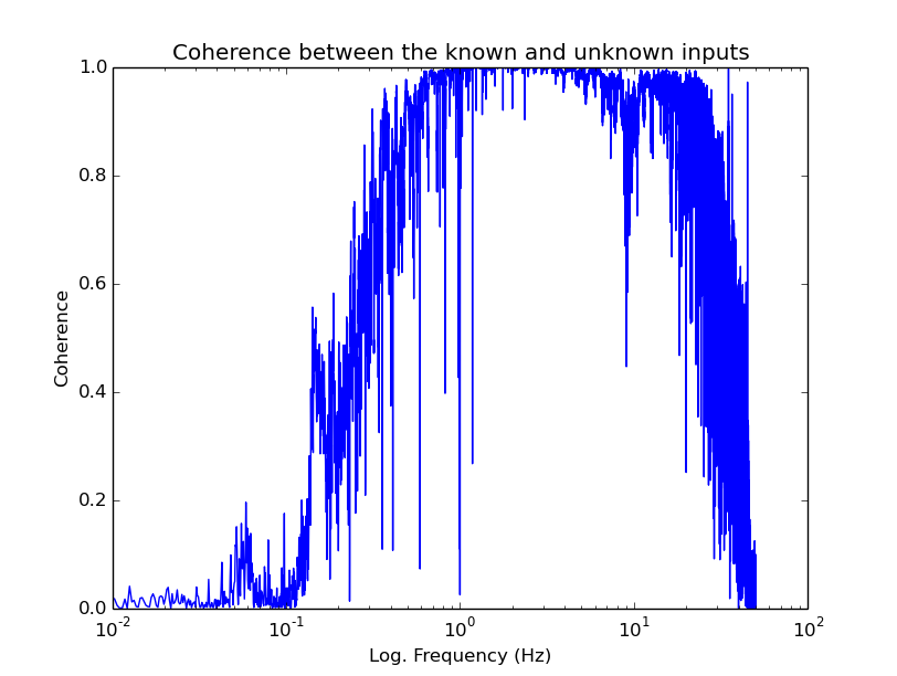
And the plot:

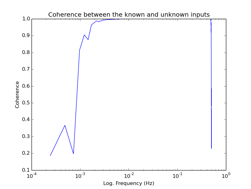
Note

Notice the excellent coherence (~1) across the entire broad band spectrum. This is critical. See Data flow & execution design more details/ explanations.

Execute:

# stage0.exe

The terminal output should be:

# stage0.exe

Stage 0: extracting epochs

Reading input data.
Truncating inputs to the overlapping time.
Extracting RESP epochs

Found a valid epoch
SEED times 2011-03-11T00:00:00.069500, 2011-03-11T23:59:59.069500
RESP epoch 2010-10-08T19:16:59, 2011-11-02T03:40:16
RESP file DATA/RESP.IU.KIP.00.LHZ
Lines 2532, 2681

Found a valid epoch
SEED times 2011-03-11T00:00:00.069500, 2011-03-11T23:59:59.069500
RESP epoch 2010-08-18T00:00:00, 2011-11-12T06:49:00
RESP file DATA/RESP.IU.KIP.10.LHZ
Lines 1610, 1766

Saving extracted epochs

Please see files
- out0.response.known for the epoch of the known instrument response
- out0.response.unknown for the epoch of the unknown instrument response

Plotting. Please wait, this may take several seconds.

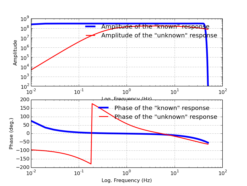
And the plot:

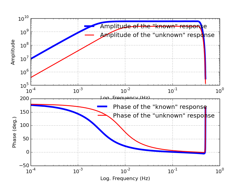
Note

Notice how the “unknown” instrument flat frequency response fits comfortably within the “known” instrument flat frequency response. This is critical. See Data flow & execution design more details/ explanations.

Execute:

# stage1e.exe

The terminal output should be:

# stage1e.exe

Stage 1: calculate transfer function
- from known input DATA/00_LHZ.512.seed
- to unknown input DATA/10_LHZ.512.seed
and restore the response for the unknown input.

Reading input data.
Truncating inputs to the overlapping time.
Determining the length of the window

Will use window length: 4096 (2**12)
Will use frequency range: [0.000122, 0.500000]

Removing DC from both input arrays.
Building prolate 4 pi window.
Calculating window's power.
Setting up temporary variables.
Allocating temporary storage.
Processing time windows:
Processing window 101 of 101.
Finished processing 101 windows.
Making exponential range of frequencies
Processing frequencies:
Processing frequency 2048 of 2048
Finished processing 2048 complex frequencies.

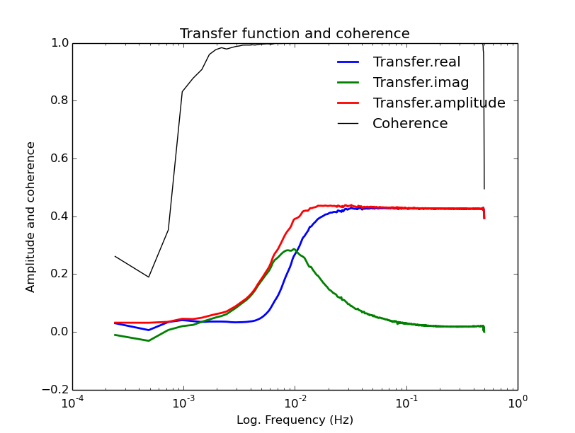
Please see the files:
- out1.coherence.npy for the coherence
- out1.frequency.npy for the frequency
- out1.transfer.npy for the transfer function

And the plot:

Execute:

# stage2.exe

The terminal output should be:

# stage2.exe

Stage 2: building and refining response.

Reading transfer function.
Reading npts and rang.
Reading known response out0.response.known
Building and saving raw unknown response
Building refined unknown response
Saving unknown response
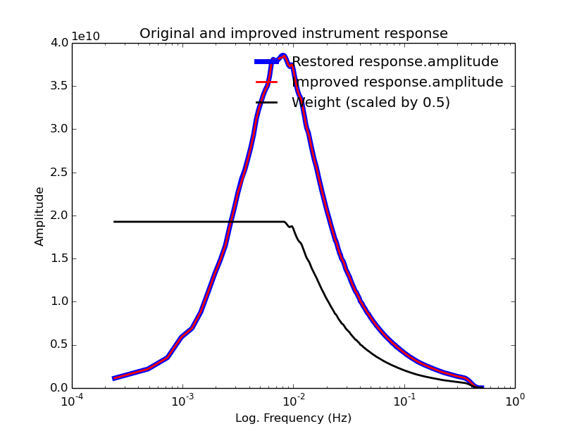
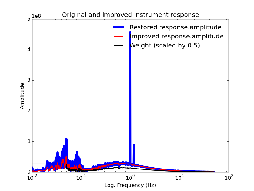
Setting weights to the amplitude (may be changed in future)

Please see files
- out2.response1.npy for the restored response
- out2.response2.npy for the improved response
- out2.weight.npy for the weight

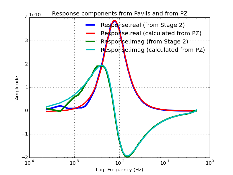
And the plot:

Execute:

# stage3.exe

The terminal output should be:

# stage3.exe

Stage 3: select the best degrees of polynomials and restore PZ

Reading data from previous stages
Selecting the best pair of M and N
Checking pair (1, 1)----------------
Possible configuration: num.of zeros, num.of poles, residual:
1, 1, 1942997487.57
Checking pair (1, 2)----------------
Possible configuration: num.of zeros, num.of poles, residual:
1, 2, 194889111.732
Checking pair (2, 2)----------------
Possible configuration: num.of zeros, num.of poles, residual:
2, 2, 170264112.775
Checking pair (3, 3)----------------
Possible configuration: num.of zeros, num.of poles, residual:
3, 3, 140575584.772
Checking pair (3, 4)----------------
Possible configuration: num.of zeros, num.of poles, residual:
3, 4, 122925219.943
Checking pair (4, 5)----------------
Possible configuration: num.of zeros, num.of poles, residual:
4, 5, 180129673.44
Checking pair (5, 5)---------------
Possible configuration: num.of zeros, num.of poles, residual:
5, 5, 274924592.053
Checking pair (6, 6)
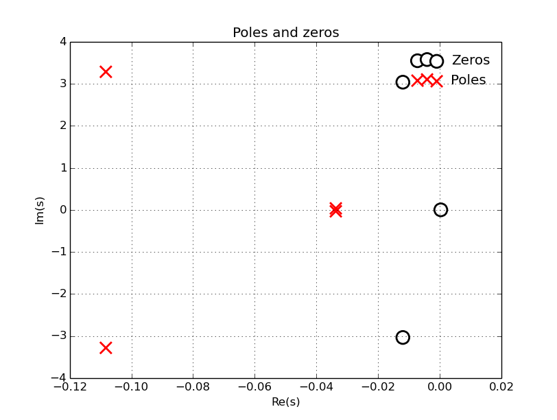
The best pair is M = 3, N = 4, MAD = 122925219.943
Zeros:
[-0.01200856+3.03657707j -0.01200856-3.03657707j  0.00028787+0.j        ]
Poles:
[-0.10827544+3.28341581j -0.10827544-3.28341581j -0.03373575+0.03510356j
 -0.03373575-0.03510356j]
Scale:
3047993562.8

Please see files
- out3.zeros.npy for the zeros
- out3.poles.npy for the poles
- out3.scale.npy for the scale
- out3.response.npy for the response restored from poles and zeros

And the plots (there are two in this stage):

Execute:

# stage4.exe

The terminal output should be:

# stage4.exe

Stage 4 - RESP file generation


Please see file out4.response.restored for the RESP formatted output

Plotting. Please wait, this may take several seconds.

And the plot:

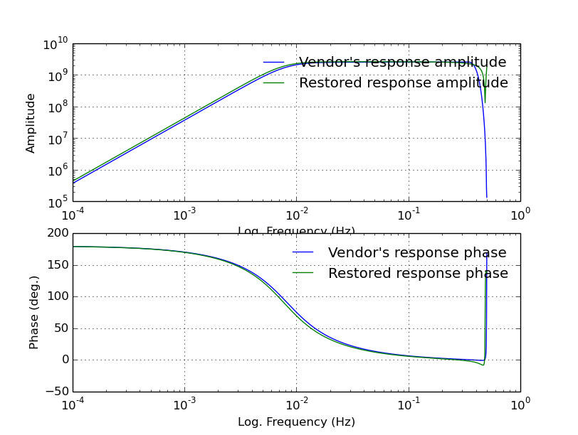
Note

The final output is a RESP-formatted instrument response file for the “unknown” sensor called out4.response.restored. It lives outside the docker container at /opt/osop/respgen/

Note

All output files live outside the docker container at /opt/osop/respgen/

Note

The “Vendor’s” response refers to the instrument response of the instrument treated as the “unknown” sensor as provided by the instrument manufacturer (or “vendor” in English) Streckeisen. The “restored” response is that generated by respGen.

Example 2: OSOP BRU2 station

Description: <1 days of 100 sps data from 2 co-located sensors, one broad band and one short-period:

(Not included by default. Available upon request)

1. “Known” instrument: a Nanometrics Trillium Compact Broadband seismometer w/ Earthdata E209 Digitizer (PA.BRU2..HHZ.D.2013.114, RESP.PA.BRU2..HHZ); and
2. “Unknown” instrument: an OSOP Sixaola (v1.2) short-period seismograph (PA.BRU4..EHZ.D.2013.114, RESP.PA.BRU4..EHZ). The response for the “unknown” Sixaola seismograph (RESP.PA.BRU4..EHZ) was generated using a shake table and the SEISAN resp program.

The Nanometrics Trillium Compact has a flat frequency response that extends to lower frequencies and, therefore, is used in this example to determine the frequency response of the more band-limited Sixaola.

Links of interest:

• Learn more about BRU2 at: http://www.osop.com.pa/hardware/seismic-vault/
• Learn more about the Nanometrics Trillium Compact at: http://www.osop.com.pa/wp-content/uploads/2014/04/sismometro-nanometrics-trillium-compact.pdf
• Learn more about the OSOP Sixaola Short-Period Seismograph: http://www.osop.com.pa/hardware/seismometer/

First, configure /opt/osop/respgen/setup.py in this way:

#!/usr/bin/env python2
UFILE = 'DATA/PA.BRU4..EHZ.D.2013.114'
KFILE = 'DATA/PA.BRU2..HHZ.D.2013.114'
URESP = 'DATA/RESP.PA.BRU4..EHZ'
KRESP = 'DATA/RESP.PA.BRU2..HHZ'
OVERLAP_FRACTION = 0.8
NUM_OF_WINDOWS = 100
LOWFRQ = 0.01
NUM_OF_POINTS = 1500
MEDIAN_LEN = 7
COHE_LIMIT = 0.6
DETERMINE_DEGREE = True
NMAX = 6
NN = 4
MM = 3
NORMFREQ = 5
ZERO_LIMIT = 0.0015

Then, execute view_cohe.exe:

# view_cohe.exe

The terminal output should be:

# view_cohe.exe

Coherence of the inputs

Input from the known instrument:
DATA/PA.BRU2..HHZ.D.2013.114

Input from the unknown instrument:
DATA/PA.BRU4..EHZ.D.2013.114

Reading input data.
Truncating inputs to the overlapping time.
Determining the length of the window

Will use window length: 262144 (2**18)
Will use frequency range: [0.000191, 50.000000]

Removing DC from both input arrays.
Calculating coherence

And the plot:

Note

In this example there is considerable less coherence between the sensors than in Example 1, but still strong coherence between the sensors in the frequency band of interest (from ~0.5 to ~0.8*Nyquist).

Execute:

# stage0.exe

The terminal output should be:

# stage0.exe

Stage 0: extracting epochs

Reading input data.
Truncating inputs to the overlapping time.
Extracting RESP epochs

Found a valid epoch
SEED times 2013-04-24T00:00:03.150000, 2013-04-24T22:43:16.500000
RESP epoch 2000-01-01T00:00:00, No ending time
RESP file DATA/RESP.PA.BRU2..HHZ
Lines 1, 1029

Found a valid epoch
SEED times 2013-04-24T00:00:03.150000, 2013-04-24T22:43:16.500000
RESP epoch 2013-01-01T00:00:00, No ending time
RESP file DATA/RESP.PA.BRU4..EHZ
Lines 1, 84

Saving extracted epochs

Please see files
- out0.response.known for the epoch of the known instrument response
- out0.response.unknown for the epoch of the unknown instrument response

Plotting. Please wait, this may take several seconds.

And the plot:

Note

Notice how the “unknown” instrument flat frequency response fits comfortably within the “known” instrument flat frequency response. This is critical. See Data flow & execution design more details/ explanations.

Execute:

# stage1.exe

The terminal output should be:

# stage1.exe

Stage 1: calculate transfer function
- from known input DATA/PA.BRU2..HHZ.D.2013.114
- to unknown input DATA/PA.BRU4..EHZ.D.2013.114
and restore the response for the unknown input.

Reading input data.
Truncating inputs to the overlapping time.
Determining the length of the window

Will use window length: 262144 (2**18)
Will use frequency range: [0.000191, 50.000000]

Removing DC from both input arrays.
Building prolate 4 pi window.
Calculating window's power.
Setting up temporary variables.
Allocating temporary storage.
Processing time windows:
Processing window 152 of 152.
Finished processing 152 windows.
Making exponential range of frequencies
Processing frequencies:
Processing frequency 131072 of 131072
Finished processing 131072 complex frequencies.

Please see the files:
- out1.coherence.npy for the coherence
- out1.frequency.npy for the frequency
- out1.transfer.npy for the transfer function

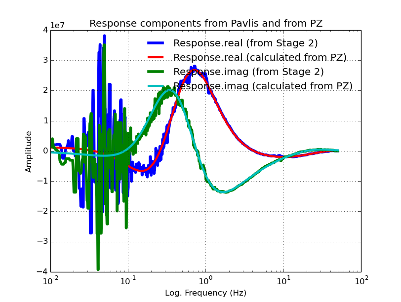
And the plot:

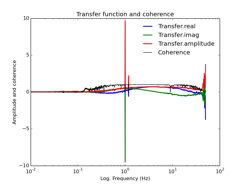
And using stage1e.exe we get:

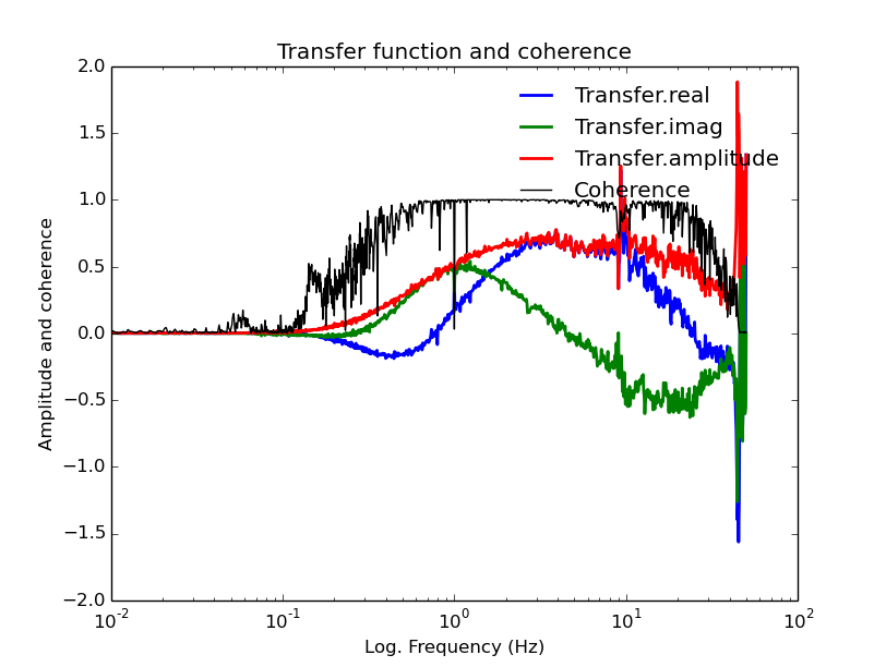
Note

stage1e (Anatoli’s linear approximation method) is better at removing transient from the data set than stage1 is (Pavlis’ robust averaging method). See Data flow & execution design for more details.

Execute:

# stage2.exe

The terminal output should be:

# stage2.exe

Stage 2: building and refining response.

Reading transfer function.
Reading npts and rang.
Reading known response out0.response.known
Building and saving raw unknown response
Building refined unknown response
Saving unknown response
Setting weights to the amplitude (may be changed in future)

Please see files
- out2.response1.npy for the restored response
- out2.response2.npy for the improved response
- out2.weight.npy for the weight

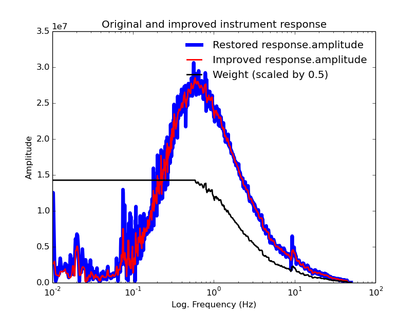
And the plot:

And using stage1e.exe we get:

Execute:

# stage3.exe

The terminal output should be:

# stage3.exe

Stage 3: select the best degrees of polynomials and restore PZ

Reading data from previous stages
Selecting the best pair of M and N
Checking pair (1, 1)----------------
Possible configuration: num.of zeros, num.of poles, residual:
1, 1, 12617699.544
Checking pair (1, 2)----------------
Possible configuration: num.of zeros, num.of poles, residual:
1, 2, 3719501.15025
Checking pair (2, 2)----------------
Possible configuration: num.of zeros, num.of poles, residual:
2, 2, 3466779.9732
Checking pair (1, 3)----------------
Possible configuration: num.of zeros, num.of poles, residual:
1, 3, 2014740.4384
Checking pair (2, 3)----------------
Possible configuration: num.of zeros, num.of poles, residual:
2, 3, 1258024.48553
Checking pair (3, 3)----------------
Possible configuration: num.of zeros, num.of poles, residual:
3, 3, 1167039.52073
Checking pair (1, 4)----------------
Possible configuration: num.of zeros, num.of poles, residual:
1, 4, 1222050.51794
Checking pair (2, 4)----------------
Possible configuration: num.of zeros, num.of poles, residual:
2, 4, 1224031.64042
Checking pair (3, 4)----------------
Possible configuration: num.of zeros, num.of poles, residual:
3, 4, 1265323.37175
Checking pair (4, 4)----------------
Possible configuration: num.of zeros, num.of poles, residual:
4, 4, 1266138.92729
Checking pair (1, 5)----------------
Possible configuration: num.of zeros, num.of poles, residual:
1, 5, 1190477.00459
Checking pair (3, 5)----------------
Possible configuration: num.of zeros, num.of poles, residual:
3, 5, 712987.694893
Checking pair (4, 5)----------------
Possible configuration: num.of zeros, num.of poles, residual:
4, 5, 660049.943494
Checking pair (1, 6)----------------
Possible configuration: num.of zeros, num.of poles, residual:
1, 6, 1250021.29066
Checking pair (2, 6)----------------
Possible configuration: num.of zeros, num.of poles, residual:
2, 6, 661938.588146
Checking pair (3, 6)----------------
Possible configuration: num.of zeros, num.of poles, residual:
3, 6, 660087.253079
Checking pair (5, 6)----------------
Possible configuration: num.of zeros, num.of poles, residual:
5, 6, 1270335.27865
Checking pair (6, 6)----------------
Possible configuration: num.of zeros, num.of poles, residual:
6, 6, 703942.863681

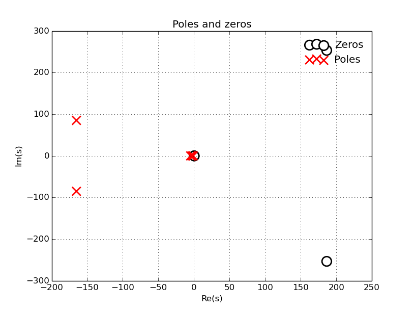
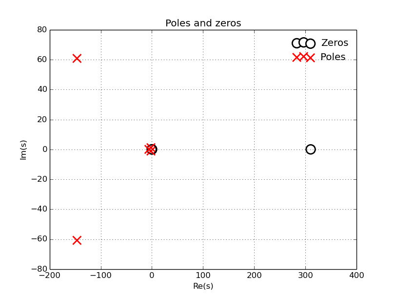
The best pair is M = 4, N = 5, MAD = 660049.943494
Zeros:
[ 186.48322108 +2.53375256e+02j  186.48322108 -2.53375256e+02j
    0.22014777 +1.89935425e-01j    0.22014777 -1.89935425e-01j]
Poles:
[-165.16834962+85.13403891j -165.16834962-85.13403891j   -4.72499488 +0.j
   -2.90319706 +0.j           -1.09210152 +0.j        ]
Scale:
74994916.8812

Please see files
- out3.zeros.npy for the zeros
- out3.poles.npy for the poles
- out3.scale.npy for the scale
- out3.response.npy for the response restored from poles and zeros

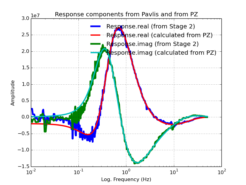
And the plots (there are two in this stage):

And using stage1e.exe we get:

Execute:

# stage4.exe

The terminal output should be:

# stage4.exe

Stage 4 - RESP file generation


Please see file out4.response.restored for the RESP formatted output

Plotting. Please wait, this may take several seconds.

And the plot:

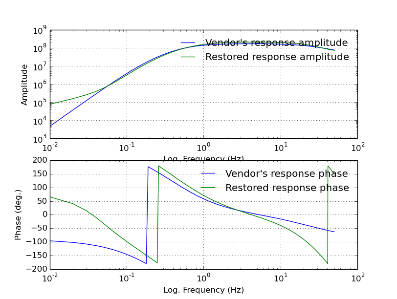
Note

The final output is a RESP-formatted instrument response file for the “unknown” sensor called out4.response.restored. It lives outside the docker container at /opt/osop/respgen/

Note

All output files live outside the docker container at /opt/osop/respgen/

Note

The “Vendor’s” response refers to the instrument response of the instrument treated as the “unknown” sensor as provided by the instrument manufacturer (or “vendor” in English) OSOP. The “restored” response is that generated by respGen.